두 지점을 잇는 연속함수, 미분가능 함수는 반드시 존재할까?

두 지점을 잇는 연속함수, 미분가능 함수는 반드시 존재할까?Math2025. 8. 28. 22:26@Ray 수학

Table of Contents

미적분학에서 두 개의 서로 다른 점이나 집합을 연결하는 함수가 반드시 존재하는지에 대한 질문은 매우 중요한 문제이다. 이 학습지에서는 연속함수(continuous function)와 미분가능함수(differentiable function)의 존재성을 보장하는 두 가지 중요한 정리를 살펴본다.

티체 확장 정리(Tietze Extension Theorem)

티체 확장 정리는 닫힌 집합(closed set)에서 정의된 연속함수를 전체 공간으로 확장할 수 있음을 보장한다.

정리: $X$가 normal space이고, $A \subset X$가 closed set일 때, $A$에서 정의된 연속함수 $f: A \rightarrow \mathbb{R}$에 대해 $F: X \rightarrow \mathbb{R}$인 연속함수가 존재하여 $F|_A = f$이다.

평면 $\mathbb{R}^2$ 위에 서로 떨어져 있는 두 개의 닫힌 원판을 생각해보자:

$A_1$: 중심이 $(-2, 0)$이고 반지름이 1인 원판
$A_2$: 중심이 $(2, 0)$이고 반지름이 1인 원판

각 원판에서 다음과 같이 함수를 정의한다:

$f(x) = 0$ for all $x \in A_1$
$f(x) = 1$ for all $x \in A_2$

거리 함수를 이용한 확장

티체 정리를 이용하면 다음과 같은 함수를 구성할 수 있다:

$$g(\mathbf{x}) = \frac{d(\mathbf{x}, A_1)}{d(\mathbf{x}, A_1) + d(\mathbf{x}, A_2)}$$

여기서 $d(\mathbf{x}, A_i)$는 점 $\mathbf{x}$에서 집합 $A_i$까지의 거리이다.

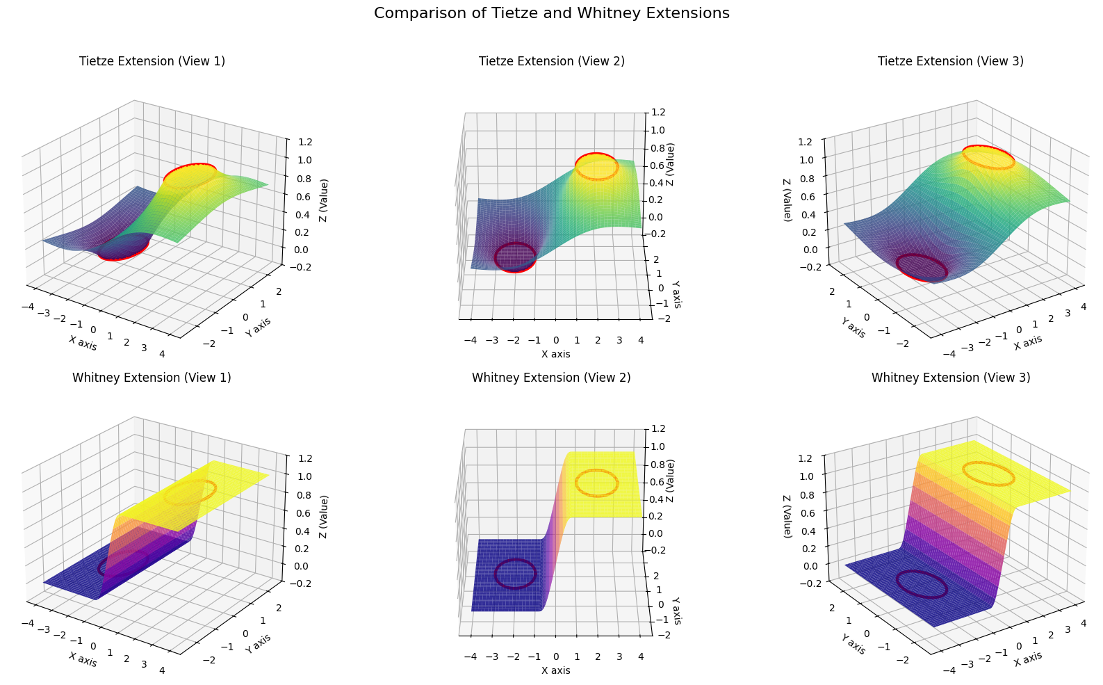
시각적 특징

연속성 보장: 함수 그래프가 끊어지지 않는다
경계에서의 각: 두 원판의 경계 근처에서 날카로운 주름(crease)이 나타날 수 있다
미분불가능성: 이러한 주름 때문에 일부 점에서 미분이 불가능하다

휘트니 확장 정리(Whitney Extension Theorem)

휘트니 확장 정리는 닫힌 집합에서 정의된 함수를 무한히 미분가능한(infinitely differentiable) 함수로 확장할 수 있음을 보장한다.

정리: $E \subset \mathbb{R}^n$이 closed set이고, $E$ 위에서 정의된 함수 $f$가 적절한 조건을 만족하면, $\mathbb{R}^n$ 전체에서 정의된 $C^\infty$ 함수 $F$가 존재하여 적당한 의미에서 $F$가 $E$ 위에서 $f$를 확장한다.

동일한 두 원판 $A_1$, $A_2$에서 같은 값을 갖는 함수를 고려한다. 휘트니 정리에 의해 구성되는 확장 함수는 매끄러운 전환 함수(smooth transition function)를 사용한다.

매끄러운 전환 함수

다음과 같은 bump function을 이용한다:

$$\phi(t) = \begin{cases}
0 & \text{if } t \leq 0 \
\exp(-1/t) & \text{if } t > 0
\end{cases}$$

이를 이용하여 매끄러운 전환을 만든다:

$$\psi(t) = \frac{\phi(t)}{\phi(t) + \phi(1-t)} \quad \text{for } t \in (0,1)$$

시각적 특징

완벽한 매끄러움: 어떤 지점에서도 각이나 주름이 없다
무한 미분가능성: 모든 차수의 도함수가 존재한다
자연스러운 전환: 두 영역 사이의 연결이 매우 부드럽다

두 정리의 핵심 차이점

특성	티체 확장 정리	휘트니 확장 정리
보장하는 성질	연속성($C^0$)	무한 미분가능성($C^\infty$)
구성의 복잡도	상대적으로 간단	매우 복잡
시각적 모습	날카로운 주름 가능	완벽하게 매끄러운 곡면
응용 분야	위상수학, 일반적인 연속성 문제	미분기하학, 매끄러운 다양체 이론

시뮬레이션 사진

import numpy as np
import matplotlib.pyplot as plt
from mpl_toolkits.mplot3d import Axes3D

# 3D 그래프 설정을 위한 함수
def setup_plot(ax, title, elev=25, azim=-55):
    """3D 그래프의 축, 제목, 시점 등을 설정합니다."""
    ax.set_xlabel('X axis')
    ax.set_ylabel('Y axis')
    ax.set_zlabel('Z (Value)')
    ax.set_title(title, fontsize=12)
    ax.view_init(elev=elev, azim=azim)
    ax.set_zlim(-0.2, 1.2)
    ax.set_facecolor('white')

# 도메인 설정: X-Y 평면
x_coords = np.linspace(-4, 4, 200)
y_coords = np.linspace(-2.5, 2.5, 200)
X, Y = np.meshgrid(x_coords, y_coords)

# 두 개의 닫힌 원판 A1, A2 정의
center1, radius1 = np.array([-2, 0]), 1
center2, radius2 = np.array([2, 0]), 1

# 1. 티체 확장 정리 예시 함수
def distance_to_disk(x, y, center, radius):
    dist_from_center = np.sqrt((x - center[0])**2 + (y - center[1])**2)
    return np.maximum(0, dist_from_center - radius)

def tietze_extension_func(x, y):
    d1 = distance_to_disk(x, y, center1, radius1)
    d2 = distance_to_disk(x, y, center2, radius2)
    denominator = d1 + d2
    return d1 / (denominator + 1e-9)

# 2. 휘트니 확장 정리 예시 함수
def smooth_step(t):
    phi = lambda val: np.exp(-1. / val) * (val > 0)
    return np.piecewise(t, [t <= 0, (t > 0) & (t < 1), t >= 1],
                        [0, lambda val: phi(val) / (phi(val) + phi(1 - val)), 1])

def whitney_extension_func(x, y):
    normalized_x = (x + 1) / 2.0
    return smooth_step(normalized_x)

# Z값 계산
Z_tietze = tietze_extension_func(X, Y)
Z_whitney = whitney_extension_func(X, Y)

# A1, A2의 경계를 그리기 위한 데이터
theta = np.linspace(0, 2 * np.pi, 100)
x_circle1 = center1[0] + radius1 * np.cos(theta)
y_circle1 = center1[1] + radius1 * np.sin(theta)
x_circle2 = center2[0] + radius2 * np.cos(theta)
y_circle2 = center2[1] + radius2 * np.sin(theta)

# 2x3 서브플롯 생성
fig, axes = plt.subplots(2, 3, figsize=(18, 10), subplot_kw={'projection': '3d'})
view_angles = [-55, -90, -125] # 세 가지 다른 시점(방위각)

# 티체 확장 그래프들
for i, azim_angle in enumerate(view_angles):
    ax = axes[0, i]
    ax.plot_surface(X, Y, Z_tietze, cmap='viridis', edgecolor='none', alpha=0.85)
    ax.plot(x_circle1, y_circle1, 0, color='red', linewidth=3)
    ax.plot(x_circle2, y_circle2, 1, color='red', linewidth=3)
    setup_plot(ax, f'Tietze Extension (View {i+1})', azim=azim_angle)

# 휘트니 확장 그래프들
for i, azim_angle in enumerate(view_angles):
    ax = axes[1, i]
    ax.plot_surface(X, Y, Z_whitney, cmap='plasma', edgecolor='none', alpha=0.85)
    ax.plot(x_circle1, y_circle1, 0, color='red', linewidth=3)
    ax.plot(x_circle2, y_circle2, 1, color='red', linewidth=3)
    setup_plot(ax, f'Whitney Extension (View {i+1})', azim=azim_angle)

fig.suptitle('Comparison of Tietze and Whitney Extensions', fontsize=16)
plt.tight_layout(rect=[0, 0, 1, 0.96])
plt.show()

시뮬레이션 영상

import numpy as np
import matplotlib.pyplot as plt
from mpl_toolkits.mplot3d import Axes3D
from matplotlib.animation import FuncAnimation

# 3D 그래프 설정을 위한 함수
def setup_plot(ax, title):
    """3D 그래프의 축, 제목, 시점 등을 설정합니다."""
    ax.set_xlabel('X a-axis')
    ax.set_ylabel('Y a-axis')
    ax.set_zlabel('Function Value (Z)')
    ax.set_title(title, fontsize=14, pad=20)
    ax.set_zlim(-0.2, 1.2)
    ax.set_facecolor('white') # 배경을 흰색으로 설정하여 가시성 높임

# 도메인 설정: X-Y 평면
x_coords = np.linspace(-4, 4, 200)
y_coords = np.linspace(-2.5, 2.5, 200)
X, Y = np.meshgrid(x_coords, y_coords)

# 두 개의 닫힌 원판 A1, A2 정의
center1, radius1 = np.array([-2, 0]), 1
center2, radius2 = np.array([2, 0]), 1

# 1. 티체 확장 정리 예시 함수 (거리 함수 이용)
def distance_to_disk(x, y, center, radius):
    """점 (x,y)에서 원판까지의 거리를 계산합니다."""
    dist_from_center = np.sqrt((x - center[0])**2 + (y - center[1])**2)
    return np.maximum(0, dist_from_center - radius)

def tietze_extension_func(x, y):
    """거리 함수를 이용한 티체 확장 함수 g(x)"""
    d1 = distance_to_disk(x, y, center1, radius1)
    d2 = distance_to_disk(x, y, center2, radius2)
    denominator = d1 + d2
    return d1 / (denominator + 1e-9)

# 2. 휘트니 확장 정리 예시 함수 (매끄러운 함수 이용)
def smooth_step(t):
    """0과 1 사이를 C-무한급으로 매끄럽게 전환하는 함수"""
    phi = lambda val: np.exp(-1. / val) * (val > 0)
    return np.piecewise(t, [t <= 0, (t > 0) & (t < 1), t >= 1],
                        [0, lambda val: phi(val) / (phi(val) + phi(1 - val)), 1])

def whitney_extension_func(x, y):
    """매끄러운 전환 함수를 이용한 휘트니 확장 함수의 예시"""
    normalized_x = (x + 1) / 2.0
    return smooth_step(normalized_x)

# Z값 계산
Z_tietze = tietze_extension_func(X, Y)
Z_whitney = whitney_extension_func(X, Y)

# A1, A2의 경계를 그리기 위한 데이터
theta = np.linspace(0, 2 * np.pi, 100)
x_circle1 = center1[0] + radius1 * np.cos(theta)
y_circle1 = center1[1] + radius1 * np.sin(theta)
x_circle2 = center2[0] + radius2 * np.cos(theta)
y_circle2 = center2[1] + radius2 * np.sin(theta)

# 그래프 그리기 및 애니메이션 설정
fig = plt.figure(figsize=(16, 8))

ax1 = fig.add_subplot(1, 2, 1, projection='3d')
ax2 = fig.add_subplot(1, 2, 2, projection='3d')

# 표면 플롯
surf1 = ax1.plot_surface(X, Y, Z_tietze, cmap='viridis', edgecolor='none', alpha=0.8)
surf2 = ax2.plot_surface(X, Y, Z_whitney, cmap='plasma', edgecolor='none', alpha=0.8)

# A1, A2 경계선 플롯 (Z=0 또는 Z=1 평면에 표시)
ax1.plot(x_circle1, y_circle1, 0, color='red', linewidth=3, label='$A_1$ Boundary')
ax1.plot(x_circle2, y_circle2, 1, color='red', linewidth=3, label='$A_2$ Boundary')
ax2.plot(x_circle1, y_circle1, 0, color='red', linewidth=3, label='$A_1$ Boundary')
ax2.plot(x_circle2, y_circle2, 1, color='red', linewidth=3, label='$A_2$ Boundary')

# 그래프 설정
setup_plot(ax1, 'Tietze Extension Example (Continuous but Not Smooth)')
setup_plot(ax2, 'Whitney Extension Example (Smooth, $C^\infty$)')

# 애니메이션 함수 정의
def animate(i):
    """각 프레임에서 카메라의 시점을 업데이트합니다."""
    ax1.view_init(elev=25, azim=i)
    ax2.view_init(elev=25, azim=i)
    return fig,

# 애니메이션 생성 및 저장
# HTML5 비디오로 저장 (jupyter/colab 환경에서 재생 가능)
anim = FuncAnimation(fig, animate, frames=np.arange(0, 360, 2), interval=50, blit=True)

# IPython.display.HTML을 사용하여 Colab/Jupyter에서 비디오 출력
from IPython.display import HTML
HTML(anim.to_jshtml())